Introduction: Understanding Infinite Solutions in a System of Linear Equations
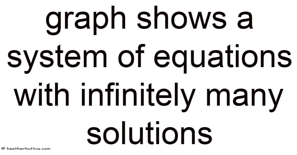
When a graph displays a system of equations with infinitely many solutions, the two (or more) lines intersect not at a single point but along an entire line. In this article we will explore why infinite solutions occur, how to identify them both algebraically and graphically, and what they mean in practical contexts. Here's the thing — recognizing this scenario is essential for students of algebra, engineers modeling real‑world phenomena, and anyone who works with linear relationships. This visual cue tells us that the equations are dependent—they represent the same line, just written differently. By the end, you will be able to interpret any graph that shows a system with infinitely many solutions and confidently explain the underlying mathematics.
1. The Geometry of a System with Infinite Solutions
1.1 Coincident Lines
On the Cartesian plane, a linear equation takes the form
[ y = mx + b ]
where m is the slope and b the y‑intercept. If two equations share exactly the same slope and the same intercept, their graphs are coincident—they lie on top of each other. Every point that satisfies one equation automatically satisfies the other, producing infinitely many common solutions.
1.2 Visual Indicators
When you look at a graph:
- Single intersection → one unique solution.
- Parallel lines → no intersection, no solution.
- Coincident lines → the lines overlap completely, indicating infinitely many solutions.
A typical graph that “shows a system of equations with infinitely many solutions” will display a single thick line (often drawn in two colors) representing both equations.
2. Algebraic Detection of Infinite Solutions
2.1 Comparing Coefficients
Consider the general linear system in standard form:
[ \begin{cases} a_1x + b_1y = c_1\ a_2x + b_2y = c_2 \end{cases} ]
If the ratios
[ \frac{a_1}{a_2} = \frac{b_1}{b_2} = \frac{c_1}{c_2} ]
hold true, the two equations are multiples of each other. The system is dependent and yields infinitely many solutions No workaround needed..
2.2 Row‑Reduction Method
Using augmented matrices, apply Gaussian elimination:
[ \left[\begin{array}{cc|c} a_1 & b_1 & c_1\ a_2 & b_2 & c_2 \end{array}\right] ]
If after elimination you obtain a row of zeros (0 0 | 0), the system has infinitely many solutions; a row of the form (0 0 | k) with k ≠ 0 would indicate inconsistency (no solution).
2.3 Example
[ \begin{cases} 2x + 3y = 6\ 4x + 6y = 12 \end{cases} ]
Dividing the second equation by 2 gives the first equation again. The coefficient ratios are
[ \frac{2}{4} = \frac{3}{6} = \frac{6}{12}= \frac12, ]
so the system has infinitely many solutions. Graphically, both equations plot the same line:
[ y = -\frac{2}{3}x + 2. ]
3. Step‑by‑Step Procedure to Identify Infinite Solutions from a Graph
- Observe the lines – Are they overlapping or merely close?
- Check slopes – Use two points on each line to calculate m. Identical slopes suggest either parallel or coincident lines.
- Check intercepts – Compare the y‑intercepts (or x‑intercepts). If they match, the lines are coincident.
- Confirm algebraically – Write the equations in standard form and test the ratio condition.
- State the solution set – Express the infinite solutions using a parameter (e.g., let x = t, then y = -\frac{2}{3}t + 2).
4. Why Infinite Solutions Matter
4.1 Real‑World Modeling
In physics, a single law may be expressed in multiple ways. Here's a good example: the equation of motion v = at + v₀ can be rearranged to at = v - v₀. Both describe the same relationship; a system built from these two forms will have infinitely many solutions because they are mathematically identical Which is the point..
4.2 Redundancy in Data
When collecting data, duplicate measurements can generate equations that are scalar multiples of each other. Recognizing infinite solutions prevents wasted effort trying to solve an over‑determined system that actually contains redundant information.
4.3 Design of Control Systems
In linear control theory, the state‑space representation may contain dependent equations. Detecting infinite solutions helps engineers reduce the model to its minimal, controllable form, improving computational efficiency.
5. Frequently Asked Questions
Q1: Can a system of three or more linear equations have infinitely many solutions?
A: Yes. If at least one equation is a linear combination of the others, the system reduces to fewer independent equations, leading to a solution space of dimension greater than zero (a line, plane, etc.). Graphically, in three dimensions you would see overlapping planes Easy to understand, harder to ignore..
Q2: What if the graph shows two lines that look almost, but not exactly, on top of each other?
A: Small visual discrepancies often stem from scaling or rounding errors. Verify algebraically: compute slopes and intercepts precisely. If the ratios of coefficients differ even slightly, the lines are distinct (parallel or intersecting at a single point) Still holds up..
Q3: Is it possible for a nonlinear system to have infinitely many solutions?
A: Absolutely. Take this: the equations x² + y² = 1 and y = √(1 - x²) describe the same unit circle, giving infinitely many points in common. Still, the visual cue differs: instead of straight lines, you’ll see overlapping curves.
Q4: How do I express the solution set when there are infinitely many solutions?
A: Use a parameter. For a two‑variable system, let one variable be free (e.g., t). Solve for the other variable in terms of t. The solution set becomes
[ {(x, y) \mid x = t,; y = -\frac{2}{3}t + 2,; t \in \mathbb{R}}. ]
Q5: Can rounding errors in calculators cause a dependent system to appear inconsistent?
A: Yes. When coefficients are large or have many decimal places, floating‑point arithmetic may produce a tiny non‑zero remainder. In such cases, treat the result as zero within an appropriate tolerance (e.g., |value| < 10⁻⁹) Worth keeping that in mind..
6. Practical Tips for Students
| Situation | What to Do | Reason |
|---|---|---|
| Graph shows two identical lines | Compute slopes and intercepts to confirm equality | Guarantees the lines are truly coincident, not just visually similar |
| Algebraic reduction yields a row of zeros | State “infinitely many solutions” and write the parametric form | Shows understanding of the solution space |
| Working with word problems | Translate the story into equations, then check if one equation is a multiple of another | Prevents unnecessary solving of a dependent system |
| Using technology (graphing calculators, software) | Zoom in on the intersection area; use the “trace” function to read exact coordinates | Helps verify that the overlap is exact, not an artifact of screen resolution |
Not obvious, but once you see it — you'll see it everywhere.
7. Extending the Concept: Infinite Solutions in Higher Dimensions
When moving beyond two variables, the geometric interpretation evolves:
- In 3‑D, each linear equation represents a plane. Two coincident planes yield infinitely many solutions forming an entire plane; three coincident planes intersect in a line (if two are the same and the third is different but shares the same line).
- In n‑D, a dependent set of equations defines a subspace of dimension n – r, where r is the rank (number of independent equations). The solution set is a linear manifold (line, plane, hyperplane, etc.).
Understanding the 2‑D case builds intuition for these higher‑dimensional scenarios, which appear in linear programming, economics, and data science Simple as that..
8. Conclusion: Turning a Visual Cue into Mathematical Insight
A graph that shows a system of equations with infinitely many solutions is more than a pretty picture; it is a direct illustration of algebraic dependence. Worth adding: by recognizing coincident lines, confirming equal slopes and intercepts, and verifying the coefficient ratios, you can confidently declare that the system has infinitely many solutions and express them in parametric form. This skill bridges visual intuition and rigorous algebra, empowering you to tackle linear systems in the classroom, the lab, and real‑world problem solving. Also, whether you are simplifying redundant data, modeling physical laws, or designing control algorithms, the ability to spot and interpret infinite solutions is a cornerstone of linear reasoning. Keep practicing with both graphs and equations, and the pattern will become second nature—turning every overlapping line into a clear, actionable insight Turns out it matters..